Here, we introduce the ionospheric storm scale called the “I-scale” [ái skéil] used in ionospheric storm plots and Classification of phenomena.
Solar flare and geomagnetic storms have clear scales determined by the X-ray flux and K-index, respectively, which explicitly represent their levels. On the other hand, the ionospheric storm has not had such a clear scale and it is difficult to represent the level of the ionospheric storm quantitatively. This is due to the large temporal and spatial variabilities in ionospheric electron density, such as seasonal, day-to-day, local time, and latitudinal variabilities.
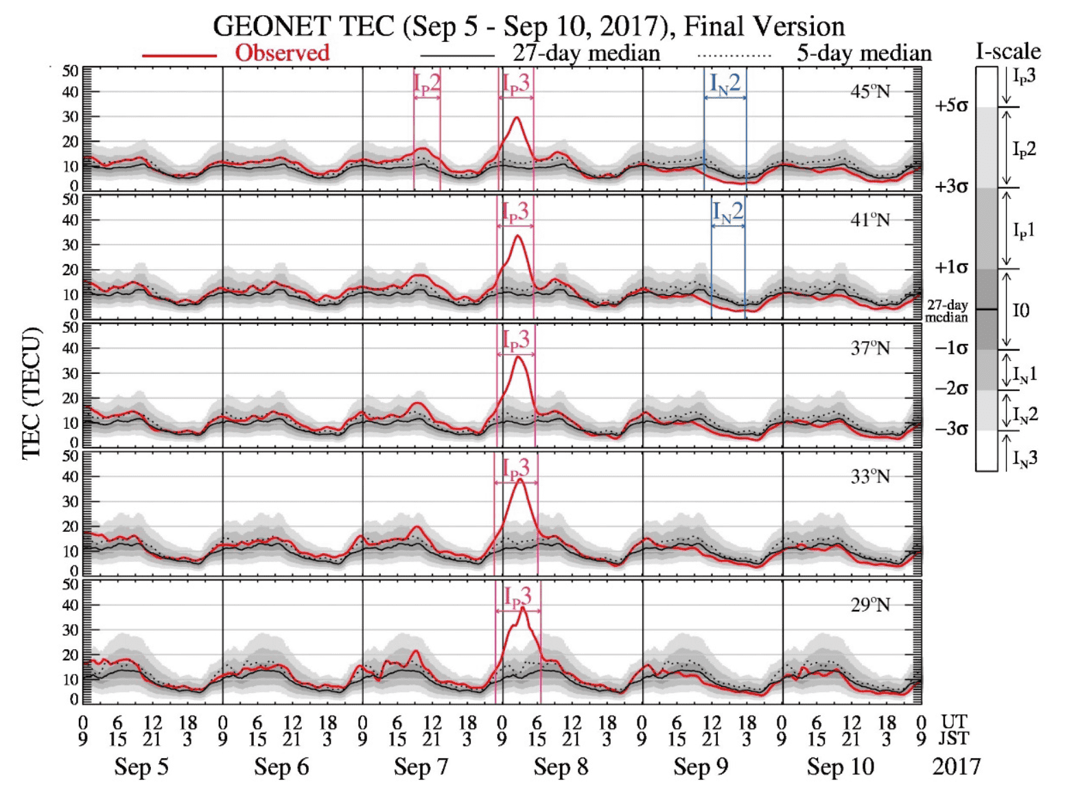
To overcome this problem and specify the level of ionospheric storm, we have developed a new ionospheric storm scale called the I-scale. The I-scale represents the relative level of deviations from the reference level, i.e., 27-day median value, compared with its standard deviation at each latitude, local time, and season over 18 years [Nishioka et al., 2017]. The I-scale is defined by setting thresholds to the normalized numbers to seven categories: I0, IP1, IP2, IP3, IN1, IN2, and IN3, as shown in Table 1. For example, IP3 corresponds to the value larger than 5σ, where σ is the standard deviation. I0 represents a quiet state, and IP1 (IN1), IP2 (IN2), and IP3 (IN3) represent moderate, strong, and severe positive (negative) storms, respectively.
We derive two I-scales on the basis of the Total Electron Content (TEC) and ionospheric F-region critical frequency (foF2). The alert level of the ionospheric storm in the website corresponds to the largest I-scale level among the TEC-based I-scales at five latitudinal bands (45, 41, 37, 33, and 29°N) and the foF2-based I-scales at four observatories (Wakkanai, Kokubunji, Yamagawa, and Okinawa).
A detailed description to derive the I-scale is as follows. Please also refer to the reference paper for more detail.
From the time-series of the ionospheric parameters O(λ, local time (LT), day), here we consider TEC and foF2, and the 27-day median value R(λ, LT, day) of the ionospheric parameters at the same LT and the same latitudinal bands (λ). We obtain the deviation ratio as
P(λ, LT, day)={O(λ, LT, day)-R(λ, LT, day)} /R(λ, LT, day).
The long-term (1997-2014) observation dataset is divided into groups according to the combination of (i) four seasons: February-April, May-July, August-October, and November-January, (ii) latitudinal bands (at five latitudes for TEC, and at four observatories for foF2), and (iii) 24 LT bins (1, 2, …, 24 hours). Then we obtain the average μ(λ, season, LT) and the standard deviation σ(λ, season, LT) values of each P-distribution group. The normalized P-distribution P is derived as
P(λ, LT, season)={P(λ, season, LT)-μ(λ, season, LT)}/ σ(λ, season, LT),
which is referred to determine the I-scale.
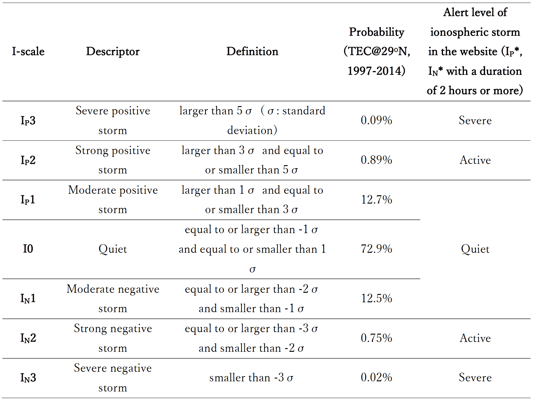
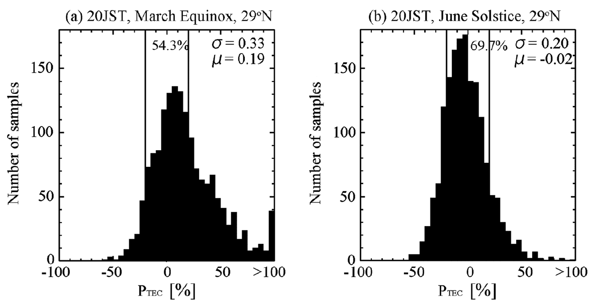
Figure 1 shows an example of the P-value distribution of TEC in the nighttime (20 JST, JST = UT+9 h) at the 29°N latitudinal band (27–31°N) over 18 years. There are significant differences between the histogram profile of P during the March equinox season (Figure 1a) and that during the June solstice season (Figure 1b). The large P-value appears more often during spring, owing to seasonal variation. Figure 2 shows similar plots using the normalized P value. The difference in the P distributions between two seasons is very small; therefore, the difference in the occurrence number of similar P values becomes smaller. Similarly, the distributions of the P value vary among different LT and latitude groups, while the occurrence number becomes similar for similar P values.
We define I-scale according to the P value as follows:
P>5 for IP3, 3<P≤5 for IP2, 1<P≤3 for IP1, -1≤P≤1 for I0, -2≤P<-1 for IN1, -3≤P<-2 for IN2, and P<-3 for IN3.
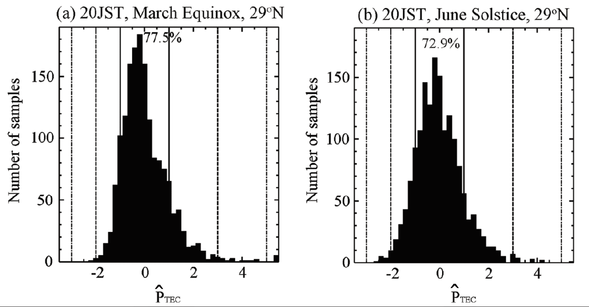
We alerts “active ionospheric storm” for positive storms with at least IP2 or negative storms with at least IN2 with a duration of 2 hours or more, and “severe ionospheric storm” for positive storms with IP3 or negative storms with IN3 with a duration of 2 hours or more over Japan. When these conditions are satisfied, flags appear in the time-series plots of TEC and foF2. Figure 3 shows the ionospheric storms seen in the TEC observation in September 2017. Severe positive storms occurred over a wide latitudinal range in Japan on September 7–8, and negative storms were detected in the high latitudes of Japan on September 9.
Reference paper:Nishioka, M., T. Tsugawa, H. Jin, and M. Ishii (2017), A new ionospheric stormscale based on TEC and foF2 statistics, Space Weather, 15, 228–239,doi:10.1002/2016SW001536. (URL for the Reference)